Breaking down JPEG compression

Mon Feb 17 2025

I recently came across this video through this tweet that explains how JPEG works.

I'll admit that even though I've used JPEG images for years, I never truly understood how they work. It's still remarkable that JPEG (introduced in 1992!) remains the most popular image format today. Its ability to maintain good image quality while keeping file sizes small has only recently faced competition from formats like AVIF and WebP, yet they still haven't come close to matching JPEG's widespread adoption.

I thought it would be fun to break down each step so I can see more clearly how it works.

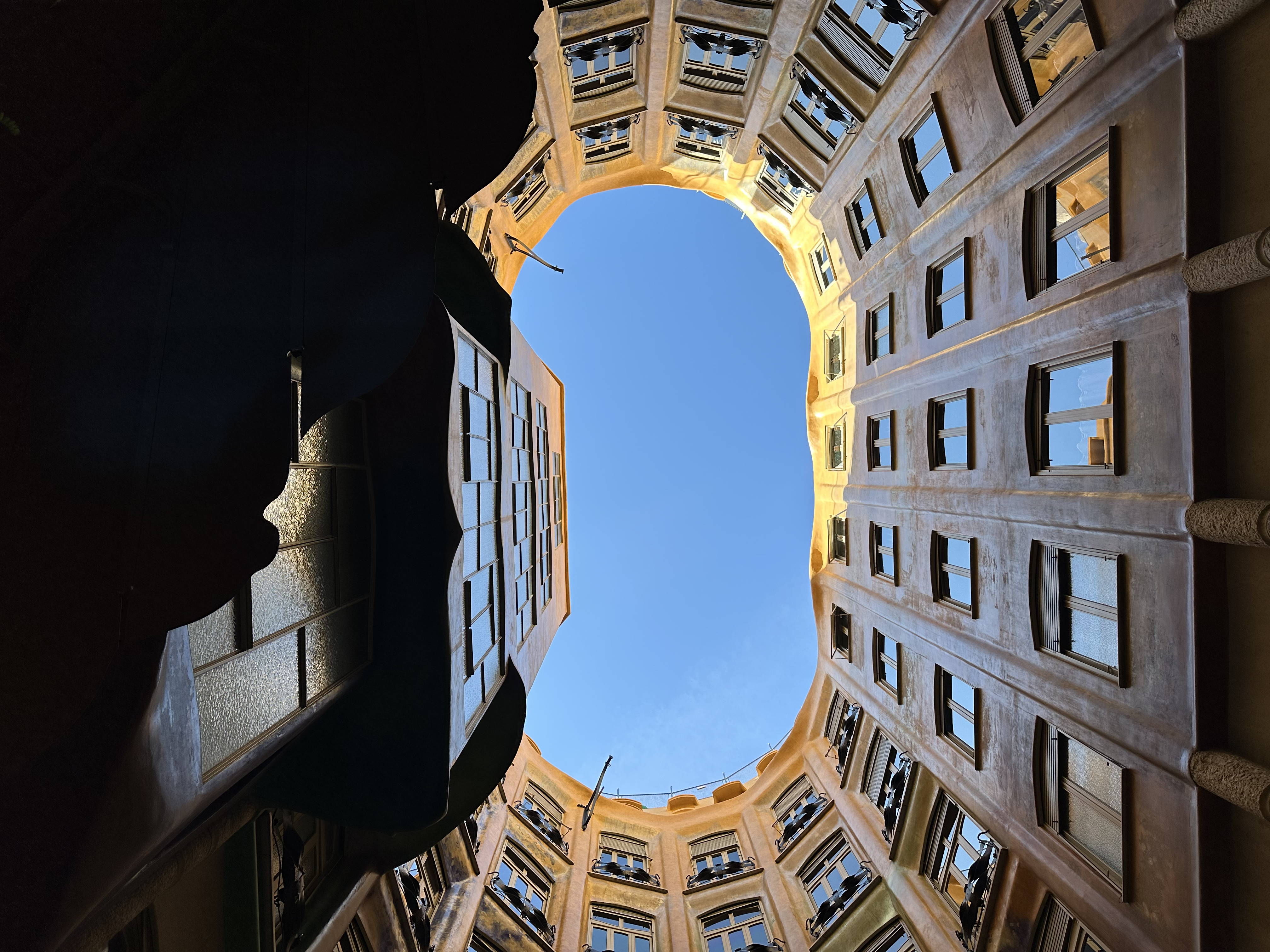
Here's the original image we will compress (a patio in Casa Mila, Barcelona by the legendary architect Antoni Gaudí btw!):

Original image

The major steps of JPEG compression are:

Color space conversion (RGB to YCbCr)
Chrominance subsampling (reduce the resolution of the chrominance channels)
Discrete Cosine Transform (DCT)
Quantization (reduce the precision of the DCT coefficients, compressing the data)
Zigzag scan (reorder the DCT coefficients in a way that makes them easier to compress)
Run-length encoding and Huffman coding (further compress the data)

Step 1: Convert the image to YCbCr color space

The first step in JPEG compression is to convert the RGB color space to YCbCr. This separation is useful because our eyes are more sensitive to changes in brightness (luminance, Y) than to changes in color (chrominance, Cb and Cr).

Y (luminance) represents the brightness of the image
Cb (blue chrominance) represents the difference between the blue component and a reference value
Cr (red chrominance) represents the difference between the red component and a reference value

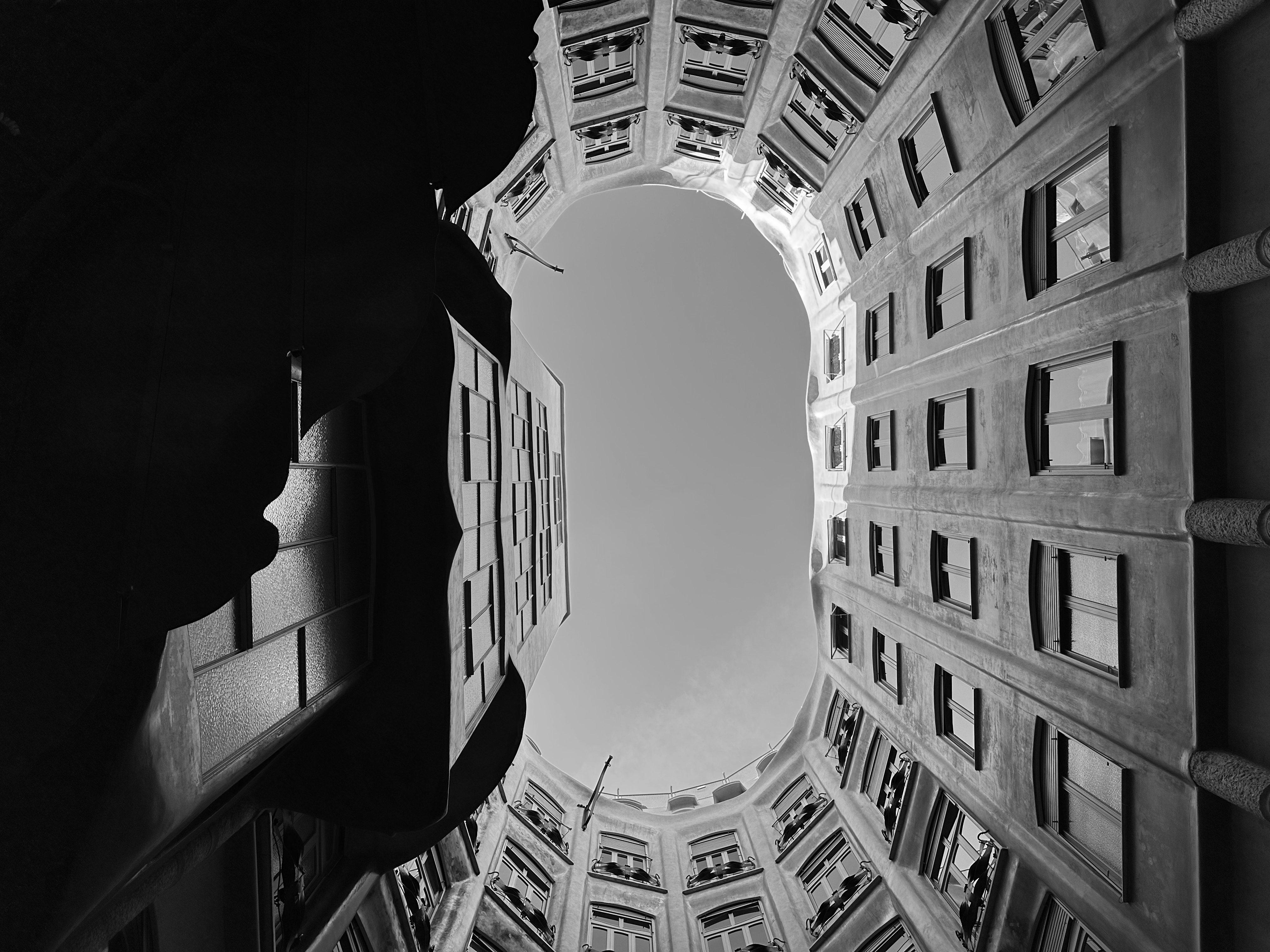
Think of it as separating a photo into brightness and color information, similar to how black and white photos capture just the brightness

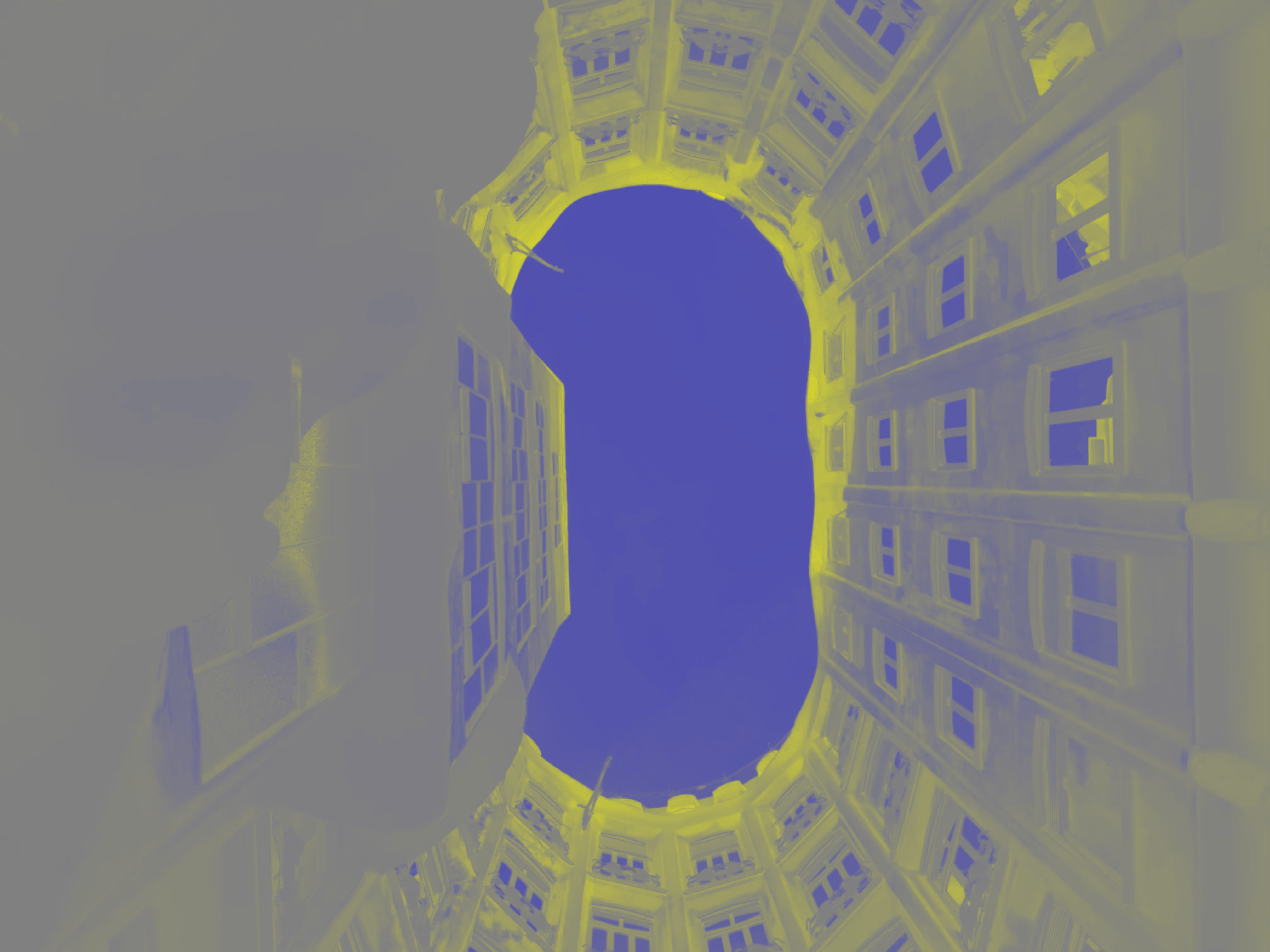
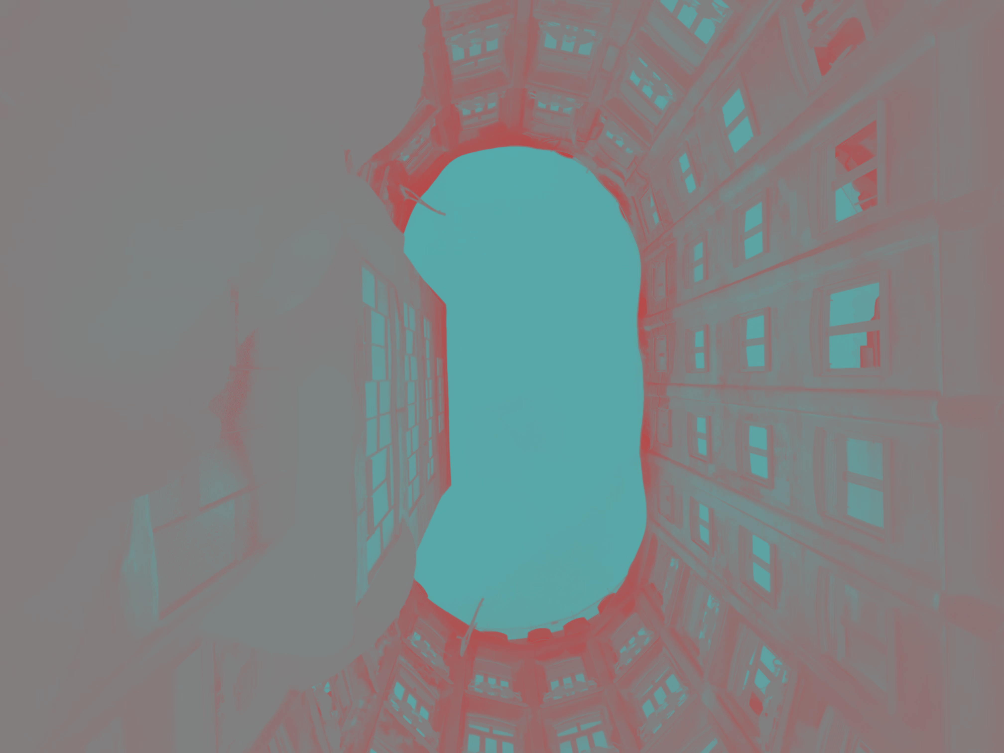
Here's how our image looks when decomposed into these three components:

Luminance (Y)

Blue chrominance (Cb)

Red chrominance (Cr)

Notice how the Y (luminance) component contains most of the detail we can recognize, while the chrominance components (Cb and Cr) contain mostly color information that appears more subtle to our eyes.

Step 2: Chrominance subsampling

Our eyes are more sensitive to luminance than chrominance. This means we can reduce the resolution of the color information without significantly affecting perceived image quality. JPEG typically uses 4:2:0 subsampling, which means we:

Keep the full resolution of the luminance (Y) component
Reduce both chrominance components (Cb and Cr) to half resolution in both horizontal and vertical directions

Here's how the chrominance components look before and after subsampling:

Original Cr

Subsampled Cr

Notice how even after reducing the chrominance resolution to 25% of the original (half in both width and height), the color information still looks quite similar.

Step 3: Discrete Cosine Transform (DCT)

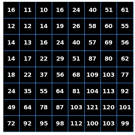
After subsampling, JPEG divides the YCrCb matrix into 8×8 blocks and applies the Discrete Cosine Transform (DCT) to each block.

The most intuitive way to understand this is that we are trying to decompose an image to a palette of "patterns". When we lay the patterns over with the appropriate brightness to each pattern, we get back the original image.

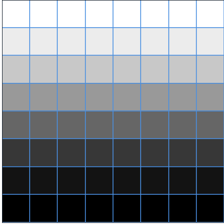
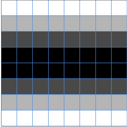
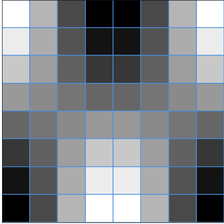
For example, here's an A-ish letter in a 8x8 grid and its DCT frequency components:

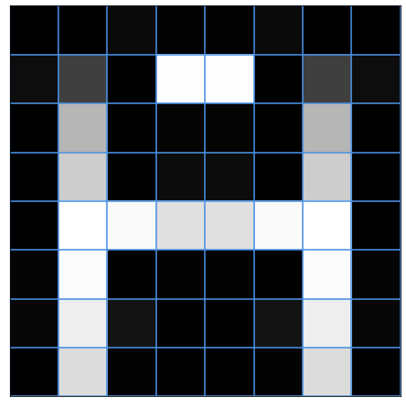
And here's the "palette of patterns" that we can use to reconstruct the original image (a 8x8 grid of DCT basis functions):

It's useful for us because we now decomposed the original A-ish letter into a combination of these patterns.

Let's look at the top 5 most significant patterns (lowest frequency patterns that our eyes are more sensitive to) that make up our letter A:

-494 x

-103 x

-209 x

-148 x

70 x

more patterns

This step is loseless, meaning we can reconstruct the original image from the DCT coefficients without any information loss.

The magic happens in the next step, where we discard the high-frequency patterns that our eyes aren't able to see that well, so we can represent the image with fewer patterns, compressing the image.

Step 4: Quantization

Quantization helps us "throw away" the least significant patterns from our DCT coefficients, so we can represent the image with fewer patterns, compressing the image. Think of it as a recipe for which patterns we keep and which we discard.

In JPEG, we have quantization matrices for each of the Y, Cb, and Cr components in different quality levels. We then divide the DCT coefficients by the quantization matrix and round to the nearest integer.

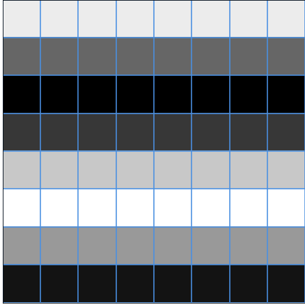
Here's an example of a quantization matrix (again, for luminance) for a quality level of 50:

Notice the values around the top left corner are smaller, so when we divide the DCT coefficients by the quantization matrix, we are keeping more of the lower-frequency patterns which are more important to our eyes. Values in the bottom right corner are larger, so when divided, the values will often be discarded.

After quantization, our DCT coefficients and resulting image look like this:

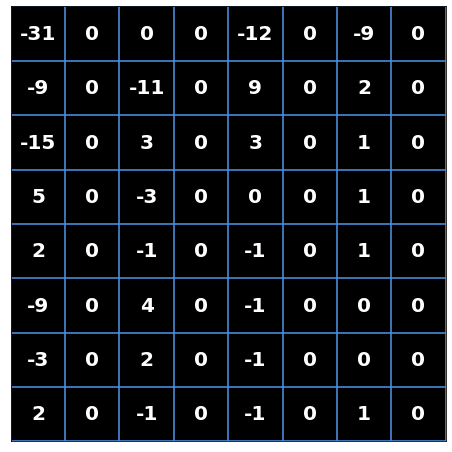
Notice almost half of the DCT coefficients are 0 now! But we can still represent the image with the remaining patterns.

Step 5: Zigzag scan

Then we reorder the DCT coefficients in a zigzag pattern, basically flattening the 2D matrix into a 1D array, sorted by increasing frequencies. Our example looks like this:

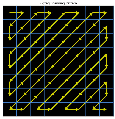
[-31, 0, -9, -15, 0, 0, 0, -11, 0, 5, 2, 0, 3, 0, -12, 0, 9, 0, -3, 0, -9, -3, 0, -1, 0, 3, 0, -9, 0, 2, 0, 0, 0, 4, 0, 2, 0, 2, 0, -1, 0, 1, 0, 0, 1, 0, -1, 0, -1, 0, -1, 0, 1, 0, 0, 0, 0, -1, 0, 0, 0, 0, 1, 0]

Step 6: Run-length encoding and Huffman coding

Then to store less information, we use run-length encoding and Huffman coding to further compress the data.

Run-length encoding basically represents consecutive zeros as a single value, so we can represent the zeroes as a list of numbers and their counts.

In our example, the run-length encoded list looks like this, format: (number_of_preceding_zeros, value):

[(-31, 0), (-9, 1), (-15, 0), (-11, 3), (5, 1), (2, 0), (3, 1), (-12, 1), (9, 1), (-3, 1), (-9, 1), (-3, 0), (-1, 1), (3, 1), (-9, 1), (2, 1), (4, 3), (2, 1), (2, 1), (-1, 1), (1, 1), (1, 2), (1, 0)]

Huffman coding assigns shorter codes to more frequent values, so we can represent the DCT coefficients as a list of numbers and their codes with fewer bits.

Altogether, for the example we have, after running both RLE and Huffman coding, we get this compression results:

Original size: 64 bytes
After RLE: 29 bytes
After Huffman: 25.4 bytes
Total compression ratio: 2.5x

And that's it!

And there we go! We then store the compressed data in a JPEG file, which contains headers and metadata like quantization tables so the decoder can decompress the image.

Demo

Here's an browser implementation of JPEG using .toBlob() to see how different quality levels affect the compression.